Test1
This clustering problem was prepared for testing if the applications are installed properly and everything works as expected. While the clustering problem is simple, it gives the possibility to demonstrate the usage of the provided applications and the auxiliary scripts.
Description of the problem
This problem contains pre-generated data set with \(N= 100 000\) samples from \(K=10\) clusters in \(d=2\) dimensional feature space. The clusters are linearly separable in the input space and the individual cluster points has Gaussian distributions around their cluster centers with the same standard deviation.
The test
After the installation of the KSC applications, the \(\texttt{tests/Test1}\) directory, under the directory specified for installation, should contain the components listed in Table 2.
File name |
Description |
|---|---|
data.tar.gz |
The pre-generated data. |
runKSCIchol_Tune.sh |
Shell script for executing the hyper parameter tuning KSC application. The script contains the, input parameter values that are appropriate for the given data set. |
runKSCIchol_Test.sh |
Same as above for out-of-sample-extension i.e. for executing the testing KSC application. |
runKSCIchol_Train.sh |
Same as above for training. |
In the following, a step by step demonstration shows how to use these scripts.
First one needs to extract the compress data directory as
bash-3.2$ tar -zxvf data.tar.gz
x data/
x data/data_Train_N10000.dat
x data/data.dat
x data/data_Labels.dat
x data/data_Valid_N10000.dat
As it can be seen, the pre-generated data set contains
File name |
Description |
|---|---|
data.dat |
The pre-generated data. |
data_Labels.dat |
The corresponding true cluster labels. |
data_Train_N10000.dat |
Sub-sample for training. |
data_Valid_N10000.dat |
Sub-sample for validation. |
As listed in Table 3, the \(\texttt{data.dat}\) file contains the whole data set: \(N = 10 000, d = 2\), dimensional samples generated from \(K = 10\) (linearly) well separated clusters. Note, that the data are standardised! The \(\texttt{data}\_\texttt{Labels.dat}\) file contains the corresponding true cluster labels while \(\texttt{data}\_\texttt{Train}\_\texttt{N10000.dat}\) and \(\texttt{data}\_\texttt{Valid}\_\texttt{N10000.dat}\) contains \(10 000\) for sub-sampled for training and validation respectively.
Since the KSC applications generates output data and their location is set to an \(\texttt{out}\) directory located in the current directory, one needs to make sure that this directory exists as
bash-3.2$ mkdir out
Before executing the provided shell script, one needs to make sure, that they are executable. This can be done by
bash-3.2$ chmod +x *.sh
Hyper parameter tuning
At this point, one could start to explore the data using the KSC application for training with the given \(\texttt{runKSCIchol}\_\texttt{Train.sh}\) script to try to find suitable range for the input parameter values such as the parameters for the incomplete Cholesky decomposition or the range of cluster number and kernel parameter values.
This has already been done, and the proper parameter values for the incomplete Cholesky decomposition as well as for the hyper parameter tuning are already set in the \(\texttt{runKSCIchol}\_\texttt{Tune.sh}\) application. Note, that the goal of the hyper parameter tuning is to find the number of clusters and kernel parameter value combination that maximises the KSC model selection criterion.
One can then execute the hyper parameter tuning KSC application with the provided script as
bash-3.2$ ./runKSCIchol_Tune.sh

 ===============================================================

 Ksc Tuning Input Parameters (with defaults for optionals):

  ------ Cholesky decomposition related:
  icholTolError              = 0.85
  icholMaxRank               = 500
  icholRBFKernelPar          = 0.002
  ------ Training data set related:
  trDataNumber               = 10000
  trDataDimension            = 2
  trDataFile                 = data/data_Train_N10000.dat

  ------ Validation data set related:
  valDataNumber              = 10000
  valDataFile                = data/data_Valid_N10000.dat

  ------ Tuning related:
  minClusterNumber           = 3
  maxClusterNumber           = 20
  kernelPrameters            = {1e-05, 1.2649e-05, ..., 1}  --> 50 number of parameters.

  ------ Clustering related:
  clEncodingScheme(BAS=2)    = 1
  clEvalOutlierThrs(0)       = 100
  clEvalWBalance(0.2)        = 0.5

  ------ Other, optional parameters:
  verbosityLevel(2)          = 2
  numBLASThreads(4)          = 4
  resFile(TuningRes)         = out/TuningRes

 ===============================================================


 ---- Starts: allocating memory for and loading the training data.
 ---- Finished: allocating memory for and loading the training data:
      ---> Dimensions of M  :(10000 x 2)

 ---- Starts: incomplete Cholesky decomposition of the Kernel matrix.
 ---- Finished: incomplete Cholesky decomposition of the Kernel matrix
      ---> Duration of ICD  : 0.13638 [s]
      ---> Final error      : 0.847978
      ---> Rank of the aprx : 110
      ---> Dimensions of G  :(10000 x 110)

 ---- Starts: allocating memory for and loading the validation data.
 ---- Finished: allocating memory for and loading the validation data:
      ---> Dimensions of M  :(10000 x 2)

 ---- Starts: tuning the KSC model.
   ---> Using Open BLAS on 4 threads.
  === KscWkpcaIChol::Tune : tuning for the 0-th kernel paraeters out of the 49
  === KscWkpcaIChol::Tune : tuning for the 1-th kernel paraeters out of the 49
  === KscWkpcaIChol::Tune : tuning for the 2-th kernel paraeters out of the 49
  .
  .
  .
  === KscWkpcaIChol::Tune : tuning for the 48-th kernel paraeters out of the 49
  === KscWkpcaIChol::Tune : tuning for the 49-th kernel paraeters out of the 49
 ---- Finished: training the KSC model
      ---> Duration         :   4.43864 [s]
      ---> The encoding(QM) :   AMS
      --->   Eta balance    :   0.5
      --->   Outlier thres. :   100
      --->   Optimality     :
             - QM value          : 0.968416
             - number of clusters: 10
             - kernel par. indx. : 20 ( = 0.0010985 )
      ---> Result is written: out/TuningRes
As it can be seen, that the application will report the input parameter values and settings, then starts the tuning. The script contains the following setting of the 2D cluster number and kernel values grid:
cluster numbers from 2 till 20
kernel parameter values: 50 values between 1.0e-05 and 1.0 in log-spaced grid
The incomplete Cholesky decomposition of the training data kernel matrix results in an approximation with a rank of 110 and the exploration of the KSC models over the 2D hyper parameter grid starts: a sparse KSC model is trained at each grid point using the training data set and evaluated on the validation set.
At the end a summary report is given, that shows the hyper parameter values of the 2D grid (cluster number of 10 and RBF kernel parameter of 0.001) that yields the highest KSC model evaluation criterion value (of 0.968) on the validation set.
The application reports the complete evaluation of the KSC models over the 2D grid by writing them into the files \(\texttt{out/TuningRes}\) (as this was set in the script). A \(\texttt{python}\) script is provided under the \(\texttt{../utils}\) directory to visualise and inspect this complete results of the KSC tuning application and can be utilised as
python ../utils/plotResTuning.py -f out/TuningRes
First, this will show a 2D (scaled) image plot of the result of the tuning over the 2D hyper parameter grid first. Then a second plot, a projection of the previous 2D plot to the cluster number scale, is shown (see more documentation of the plotResTuning script). The resulted figures are shown in Fig. 2 and Fig. 3.
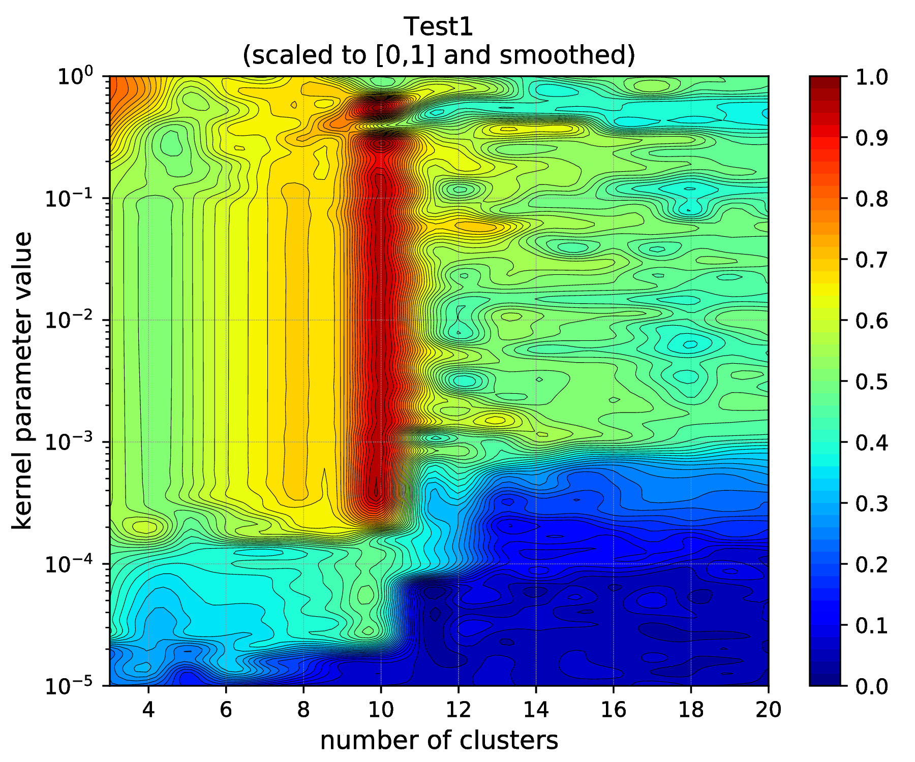
Fig. 2 Results of the KSC hyper parameter tuning application (2D image as visualised by using the plotResTuning script).
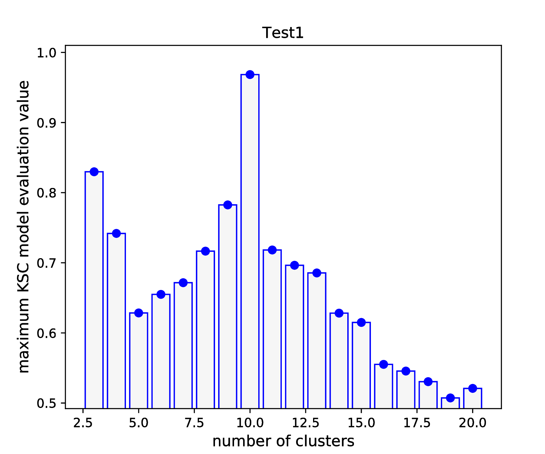
Fig. 3 Results of the KSC hyper parameter tuning application (1D projection as visualised by using the plotResTuning script).
According to the results shown in Fig. 2 and Fig. 2, there is a clear maximum of the KSC model selection criterion (AMS) value at cluster number 10. Moreover, according to the results shown in Fig. 2, this maximum value can be achieved with a wide range (\(\sim 2\times 10^{-4} - 2\times 10^{-1}\)) of RBF kernel parameter value. These results confirm the optimality point reported at the end of the KSC tuning application: optimal number of cluster is 10 and optimal RBF kernel parameter value is 0.001.
Out-of-sample extension i.e. testing
After determining the optimal values of all the necessary input parameters, one can train the sparse KSC model on the training set and apply the trained model to cluster any further, unseen data. This can be done by using the KSC application developed for testing. The \(\texttt{runKSCIchol}\_\texttt{Test.sh}\) script, already contains the appropriate values of all the input parameters of this application, including the optimal cluster number and RBF kernel parameter values, determined above during the hyper parameter tuning. Therefore, one can execute the application by
bash-3.2$ ./runKSCIchol_Test.sh

 ===============================================================

 Ksc Training & Testing Input Parameters (with defaults for optionals):

  ------ Cholesky decomposition related:
  icholTolError              = 0.85
  icholMaxRank               = 500
  icholRBFKernelPar          = 0.002

  ------ Training data set related:
  trDataNumber               = 10000
  trDataDimension            = 2
  trDataFile                 = data/data_Train_N10000.dat

  ------ Test data set related:
  tstDataNumber              = 100000
  tstDataFile                = data/data.dat

  ------ Clustering related:
  clNumber                   = 10
  clRBFKernelPar             = 0.001
  clEncodingScheme(BAS=2)    = 1
  clEvalOutlierThrs(0)       = 100
  clEvalWBalance(0.2)        = 0.5
  clResFile(CRes.dat)        = out/CRes.dat
  clLevel(1)                 = 1

  ------ Other, optional parameters:
  verbosityLevel(2)          = 2
  numBLASThreads(4)          = 4

 ===============================================================


 ---- Starts: allocating memory for and loading the training data.
 ---- Finished: allocating memory for and loading the training data:
      ---> Dimensions of M  :(10000 x 2)

 ---- Starts: incomplete Cholesky decomposition of the Kernel matrix.
 ---- Finished: incomplete Cholesky decomposition of the Kernel matrix
      ---> Duration of ICD  : 0.136879 [s]
      ---> Final error      : 0.847978
      ---> Rank of the aprx : 110
      ---> Dimensions of G  :(10000 x 110)

 ---- Starts: training the KSC model.
   ---> Using Open BLAS on 4 threads.
          ====> Starts computing eigenvectors...
   ---> Using Open BLAS on 4 threads.
          ====> Starts forming the Reduced-Reduced and Reduced-Test kernelmatrix...
          ====> Starts computing the reduced set coefs...
          ====> Starts generating encoding...
 ---- Finished: training the KSC model
      ---> Duration         : 0.05619 [s]
      ---> The encoding(QM) : AMS
      --->   Quality value  : 0.95821
      --->   Eta balance    : 0.5
      --->   Outlier thres. : 100


 ---- Starts: allocating memory for and loading the test data.
 ---- Finished: allocating memory for and loading the test data:
      ---> Dimensions of M  :(100000 x 2)

 ---- Starts: clustering the test data with the KSC model.
   ---> Using Open BLAS on 4 threads.
 ---- Finished: test data cluster assignment
      ---> Duration         : 0.167816 [s]
      ---> The encoding(QM) : AMS
      --->   Quality value  : 0.999999
      --->   Eta balance    : 0.5
      ---> Result is writen :
      --->   Clustering     : out/CRes.dat
Similarly to the tuning, the KSC application developed for out-of-sample extension also reports the input parameter values and configurations. The process starts with the training of the sparse KSC model on the training set, including the ICD of the corresponding kernel matrix. One can see that ICD and the training of the KSC model takes 0.14 and 0.06 [s] in this case respectively. Then the trained KSC model is applied on the whole (\(N = 100 000\)) data set and the clustering results (i.e. the labels) are saved into the \(out/CRes.dat\) file (as set in the script).
Clustering the complete data set with its \(N = 100 000\) points took 0.17 [s] while the clustering result (according to the reported model selection criterion value of 0.99999) is perfect. One can utilise the evaluateClusteringRes.py (located under \(\texttt{../utils/}\)) script to compute the corresponding adjusted rand index (ARI) as
bash-3.2$ python ../utils/evaluateClusteringRes.py -c out/CRes.dat -t data/data_Labels.dat
==== (Python) === : Evaluating clustering result ...
  ---- (Python) --- : Computing Adjusted-Rand-Score ...
   ===> The Adjusted Rand-Score =  1.000
The ARI = 1.0 also confirms that the clustering of all the \(N = 100 000\) data point is perfect (which can be only because the 10 clusters are separable).
The plotClusteringRes.py (located under \(\texttt{../utils/}\)) script can be used for plotting the result as
bash-3.2$ python ../utils/plotClusteringRes.py -d data/data.dat -l out/CRes.dat
 ==== (Python) === : visualising the result of the clustering...
This should generate the figure shown in Fig. 4.
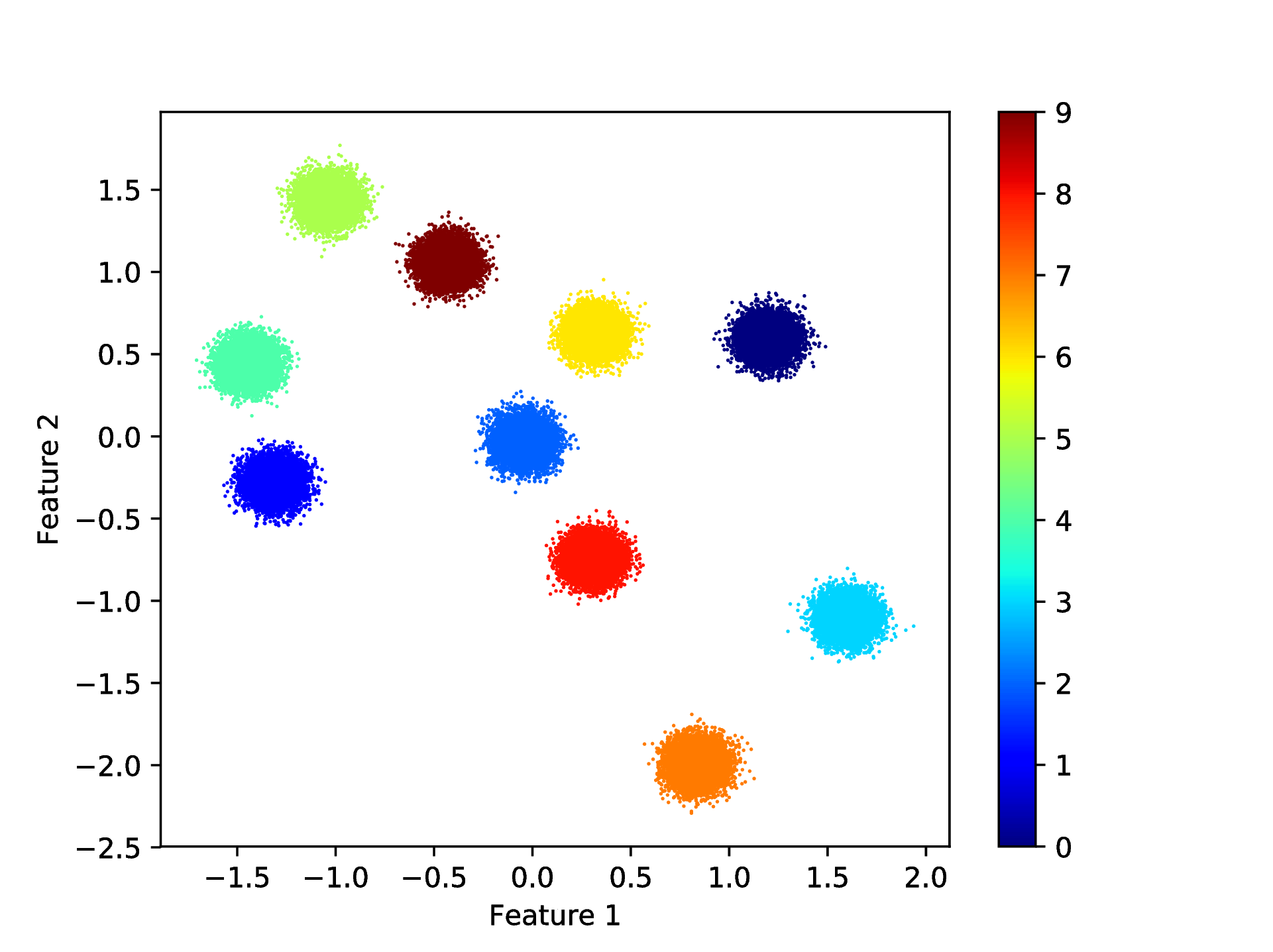
Fig. 4 Results of the KSC test (out-of-sample extension) application when clustering the whole Test1 data set.